Do you often need to do linear interpolation in Excel from a table of values? Does it bother you a hell of a lot that some people choose a value in between instead of doing a linear interpolation? Do you like having intricate formulas in your Excel that nobody else know what they do? Do you want to become an Excel Wizard?
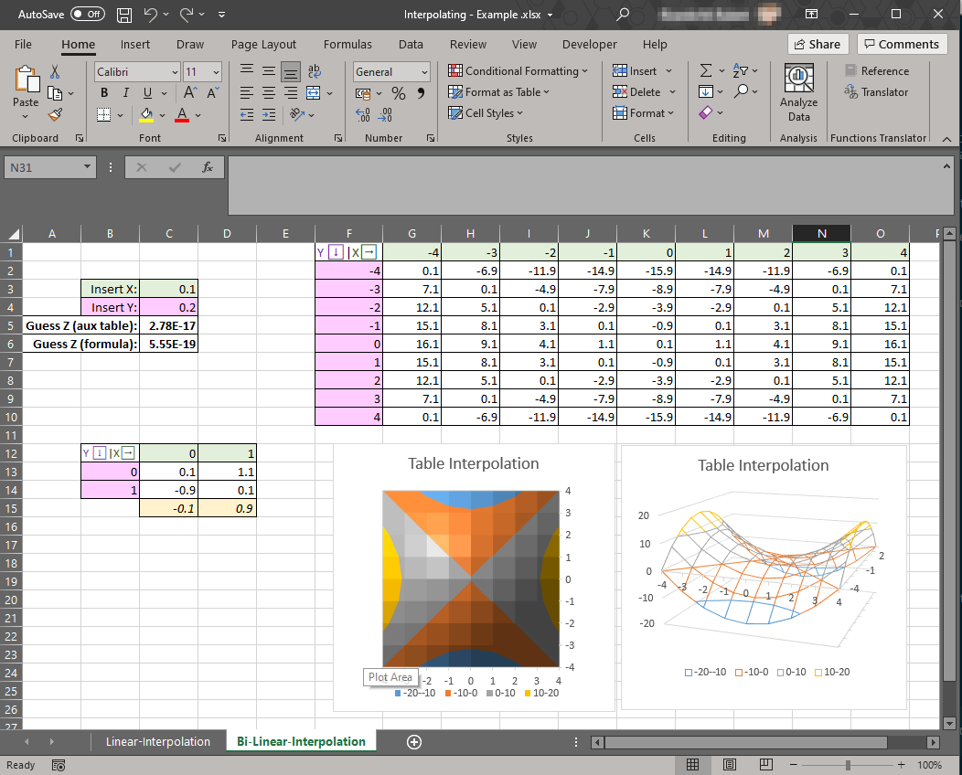
Figure 1: Screenshot of the template
Any sensible person would have replied Yes to the last three questions. However, only people working in (Civil) Engineering reply Yes to the first question. Why? You would ask. Well, because in Civil Engineering (and its associated branches like hydraulic, Geotech, etc…) we have accepted that the world is not ruled by formulas, but from a set of empiric values done in a study on the XX or the XIX century. Those studies drew their conclusions in the form of a graphical table, a numerical table or if we were lucky, a statistical regression formula that fit the original data fairly well.
And because I was pissed off with the table/figure looking to retrieve values I decided to create an excel able to do so automatically for me. And here it is the definitive1 Excel to perform Linear Interpolation (single entry tables) and Bilinear Interpolation (Double entry tables). You can download it from here , or keep reading to know more about how it works.
Linear Interpolation
It would be great if Excel had a linear interpolation function, but it doesn’t. Excel has the =FORECAST.LINEAR(X,knownY,knownX) function. But this formula will use the whole set of data to create a linear regression model. This is not what we want.
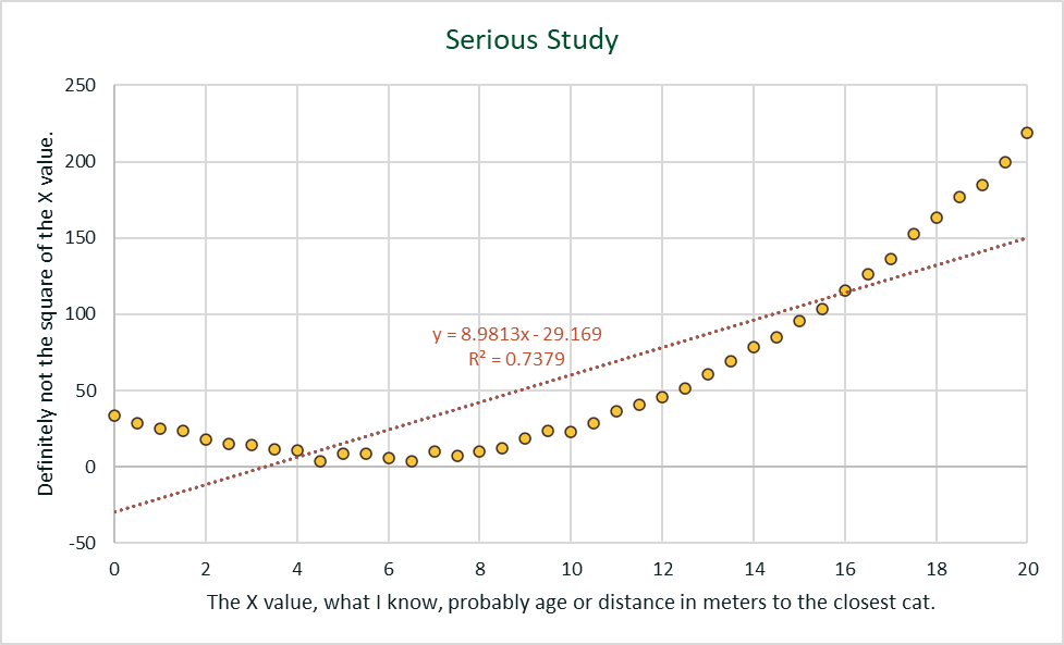
Figure 2: A typical linear regression model that could be seen in some articles.
So to work as we want, we need to filter it. We use the =OFFSET() and =MATCH() functions to select only a pair of points. After filtering, we have only 2 points, and a linear regression model of two points is indeed a linear interpolation2.
The formula used is below, remind to delete all new lines if you copy and paste it.
    =FORECAST.LINEAR(<X>,OFFSET(<headerX>,MATCH(<X>,<knownXrange>,1),
      <columnknownY>,2,1),OFFSET(<headerX>,MATCH(<X>,<knownXrange>1),0,2,1))
Where:
<X>is the cell of the x value we need to guess,<headerX>is the column name of the known X values,<knownXrange>is the range of the known X values, and,<columnknownY>is an integer number of where the known Y values are located. If they are the next (➡) column to X it will be 1. Two columns to the right = 2, etc…
There is an additional use, you can use this formula to convert any set of values into an equally spaced (in X) set of values. If you do so, be careful as the local and global extreme values will be removed.
Bilinear Interpolation
I also have added a bilinear interpolation. Bilinear interpolation might not be as intuitive as linear interpolation. A quick read to this Wikipedia Article might be helpful, alternatively, you can look at the image below from the very same article. As you can see, one needs to perform 3 linear interpolations with the data on the table to get the required result.
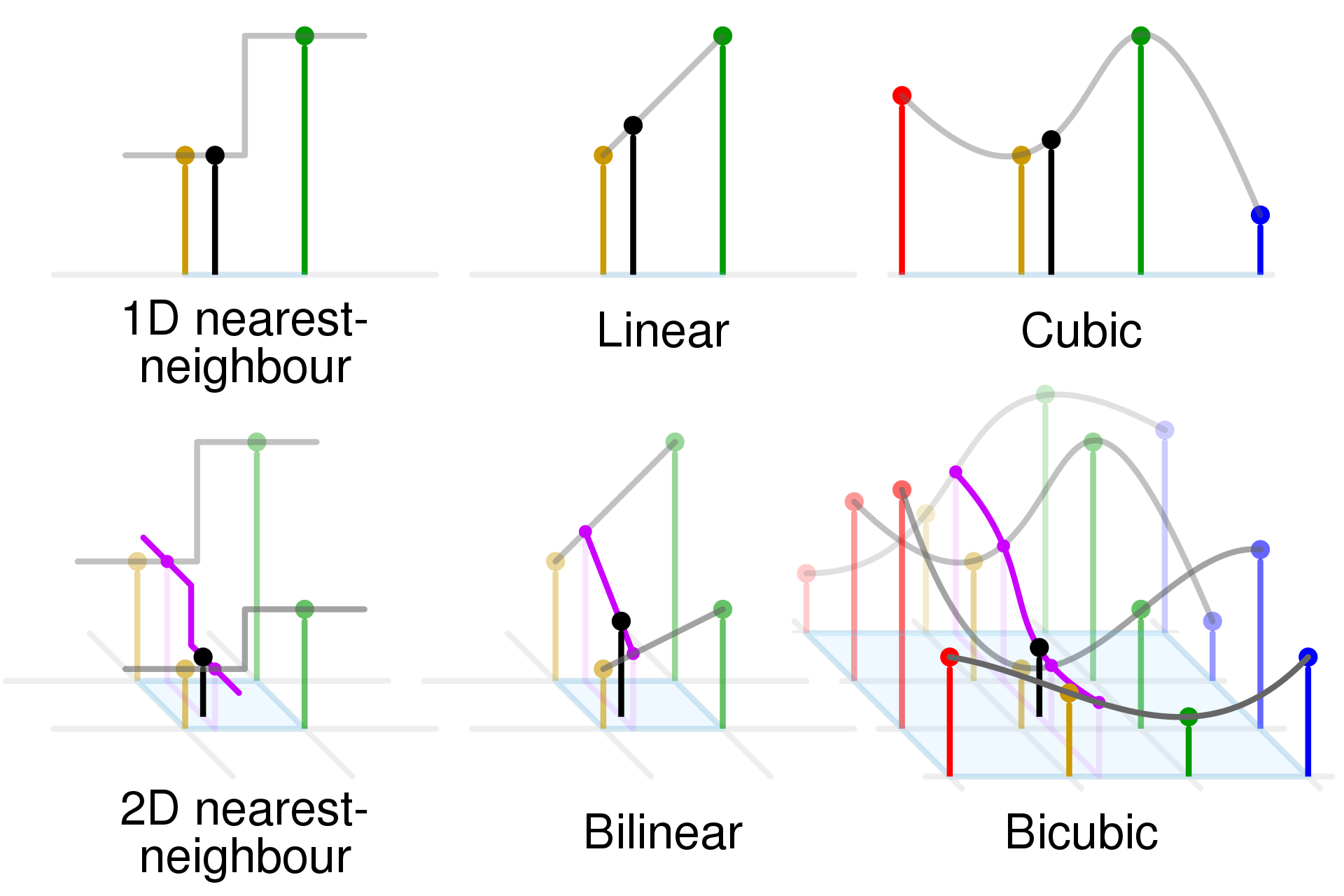
Figure 3: Comparison of Bilinear interpolation with some 1- and 2-dimensional interpolations
On my Excel template, I have done this in 2 different ways. The first way, I use an auxiliary table. In this table, the 4 values are identified using the offset and match functions. Then the 3 linear interpolations are performed using the =FORECAST.LINEAR() function and voilà! we have our result. This solution is neat, easily auditable but takes space, exactly 3x2 cells for the auxiliary table.
There is another solution that is to use the following formula from the aforementioned wiki article:
\[ f(x, y) = a_{00} + a_{10}x + a_{01}y + a_{11}xy \]
Where:
- \(a_{00} = f(0, 0)\),
- \(a_{10} = f(1, 0) - f(0, 0)\),
- \(a_{01} = f(0, 1) - f(0, 0)\), and,
- \(a_{11} = f(1, 1) - f(1, 0) - f(0, 1) + f(0, 0)\).
Which when translated to Excel become this monster (I have divided into lines for clarity, remove them before using in Excel):
=OFFSET(<topleftTableHeader>,MATCH(<Y>,<knownY>,1),MATCH(<X>,<knownX>,1),1,1)+
 (OFFSET(<topleftTableHeader>,MATCH(<Y>,<knownY>,1),MATCH(<X>,<knownX>,1)+1,1,1)-
 OFFSET(<topleftTableHeader>,MATCH(<Y>,<knownY>,1),MATCH(<X>,<knownX>,1),1,1))*<X>+
 (OFFSET(<topleftTableHeader>,MATCH(<Y>,<knownY>,1)+1,MATCH(<X>,<knownX>,1),1,1)-
 OFFSET(<topleftTableHeader>,MATCH(<Y>,<knownY>,1),MATCH(<X>,<knownX>,1),1,1))*<Y>+
 (OFFSET(<topleftTableHeader>,MATCH(<Y>,<knownY>,1)+1,MATCH(<X>,<knownX>,1)+1,1,1)-
 OFFSET(<topleftTableHeader>,MATCH(<Y>,<knownY>,1),MATCH(<X>,<knownX>,1)+1,1,1)-
 OFFSET(<topleftTableHeader>,MATCH(<Y>,<knownY>,1)+1,MATCH(<X>,<knownX>,1),1,1)+
 OFFSET(<topleftTableHeader>,MATCH(<Y>,<knownY>,1),MATCH(<X>,<knownX>,1),1,1))*<X>*<Y>
Where:
<X>is the cell of the X value we need to guess,<Y>is the cell of the Y value we need to guess,<knownX>is the range of the known X values (X values have to go from left to right),<knownY>is the range of the known Y values (Y values have to go from top to bottom), and,<topleftTableHeader>is the top-left header of the table with the data.
This solution is a nightmare to audit but hey, it takes only one cell!
Don’t forget to download the excel.
Acknowledgments
Figure 3 is from Cmglee, CC BY-SA 4.0.